Explaining "Not-QE"

A summary of this post can be found here.

As there has been a constant debate about what to make of the latest interventions by the Federal Reserve (FED), whether we can call it QE or "Not-QE",  I thought it could be appropriate to try to explain, why we can technically argue that this is not a QE. To understand this, it is essential not only to understand what the FED or any other Central Bank does but to understand how monetary policy is implemented and how it has evolved since the Global Financial Crisis (GFC)

Many may know that the FED tries to control short-term rates (important emphasis on SHORT-TERM rates) by setting a Federal Funds Target Rate. The federal funds market is an interbank market where banks and other institutions trade federal funds (bank reserves) on unsecured (no collateral pledged) basis. It is important to note, that the FED only sets a target rate or a target range and the actual prevailing rate is the weighted average of unsecured loans issued in the private interbank market. The actual rate is called the Effective Federal Funds Rate (EFFR). The idea of why lowering short-term rates is supposed to work in spurring activity is that as the short-term interbank rate is lowered, the yield curve steepens, so that the spread between short and long rates will grow. As banks make money through maturity transformation (by borrowing short and lending long), this spread will increase their profitability and induce more competition and concomitantly pushing even longer-term rates lower. This is supposed to increase customer demand (borrowing) and with this, economic activity and inflation (another mandate of the FED is to provide full employment). However, as we get closer to the zero-lower bound (nominal federal funds rate = 0), this orthodox theory will get more complex. This is why many unconventional methods were taken during the GFC. The issue was (and is) that because the real aim of FED is to induce lending by reducing real federal funds rates (r*), which is calculated as the nominal rate (i) – inflation (π). Lowering of r* becomes difficult when nominal rates are tied to zero. With nominal rates at zero and inflation expectations lowering, it becomes an automatic tightening process, with real rates increasing (tightening) with every inch of a drop in inflation expectations (i-π=r*). Extremely, this could mean a tightening loop, which materializes as a deflationary spiral further exacerbating the problem. This is of course if we are to believe, as it is in the mainstream, that deflation is automatically a scenario of death and doom. For a credit-based monetary system, this argument is quite solid.

So now that we have gone through the basic description of FED’s actions, the questions stand, how does the FED actually implement this policy? To reflect on the issues of today (repo intervention), we need to go back to a time prior to GFC and study the previous monetary policy implementation method; the corridor system. For some strange reason, by my knowledge, it is still taught in many graduate textbooks as a prevailing system, even if it hadn’t existed for the last 10 years. 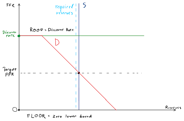The corridor system is a policy implementation method where there are three factors, a floor or the zero lower bound (or deposit rate set at 0%), a roof, or the discount window (primary credit rate, or actually three different rates) and reserve scarcity. The zero-lower bound is supposed to work as a floor as below a zero-nominal rate, people should rather be holding cash than deposits (of course with the actual inconvenience of holding cash in great quantities, the rate can technically be slightly below 0). The roof, or the discount window, is a “no-questions-asked” lender-of last resort lending channel, where the FED stands ready to supply reserves in any amount required against eligible collateral. As this is a loan (= asset for the FED), it also means that when the banks are to rely on discount window loans, it will expand FED’s balance sheet unless sterilized (by a countering measure such as selling T-Bills). This is what initially got the FED shifted from a corridor system into a floor system, of which I will explain more below.

Reserve scarcity. Bank reserves are bank deposits held by depository institutions (banks) at the FED. Only the balances held in these deposit accounts are counted as bank reserves. Other institutions holding accounts at the FED include Government Sponsored Enterprises or GSE’s (such as Fannie Mae, Freddie Mac, and Federal Home Loan Bank), foreign central banks and other foreign institutions (such as Bank of International Settlements) and the US Treasury with its Treasury General Account (TGA). All money (reserves) that is transferred from these banks holding a FED account to one of the other institute accounts DISAPPEARS from the banking system. The money that “disappears” is money less to do interbank transactions with. This means e.g. that all tax payments and the money got from US treasury debt issuances that are transferred to TGA disappear from the banking system. The US government is also having accounts at individual banks themselves with Treasury Tax and Loan program or TT&L, transfers to these accounts do not affect reserve balances.

The reserve scarcity is an important characteristic of the pre-GFC monetary policy implementation method. When there is a scarcity of reserves in the banking sector, even minor increases or decreases in the supply will affect the prevailing federal funds rate. The reserve balances were usually just slightly above the level required in aggregate by reserve requirements, the need for slight excess resulting from a need to prepare for sudden unexpected overdrafts on reserve accounts. The more reserves in excess to what is required there are in the banking system, the lower the resulting interest rate will be, given no other tools are used to counter this drop.

When in a corridor system, the FED set its target for Federal Funds rates and the actual Effective Federal Funds Rate was achieved by an ACTIVE and DAILY management of reserve balances using the FED’s System Open Market Account (SOMA) portfolio, the asset portfolio FED had to conduct its operations with. These operations are called Open Market Operations (OMO) and are done with a Primary Dealer (PD) as a counterparty or intermediate player.  An interesting side note here is that all PDs are mandated by LAW to buy US Treasuries in a Treasury auction and thus conveniently for the US Government there is always a demand for its debt securities. Although this is the case, there is still plenty of reasons for the PDs to happily be the counterparty here, as the US government debt obligations are deemed the most pristine collateral in the banking system, facilitating great chunk of financial institutions funding. When the FED conducted OMOs, they either used Repurchase Agreements (repo) or purchase of assets to increase the supply of reserves (and thus the amount of reserves left for the banking sector to lend in the private market) or Reverse Repurchase Agreements (reverse repo) or sales of assets to decrease the supply of reserves. Repurchase Agreement or a repo is an operation where one sells an asset in exchange for money with a contract to buy it back e.g. the next day. Repo can be thought more simply as a short-term collateralized borrowing. Reverse Repurchase Agreement is an operation where one buys an asset with a contract to sell it back e.g. the next day or more simply it is short-term collateralized lending. For some strange reason, the FED calls its repo operations from the perspective of the receiving party, i.e. for the FED, repo = lending (liquidity increasing as it increases reserves) and reverse repo = borrowing (liquidity reducing as it reduces reserves).Another point to “strike home” with regards to repo is its temporary nature (unless rolled over) unlike, say, an asset purchase which is permanent until reverse action is made. The active reserve management operations done by FED during a corridor system were mostly repo’s (short-term) and included T-Bills (short term US debt with a maturity of <1 year), meaning that the OMO’s were always done with collateralized- or secured-basis to manage unsecured federal funds rates (no collateral).  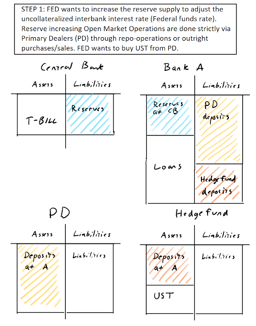An important feature of this system was, that the interbank market was an active market where funds were allocated actively to needing parties, this is not the case in a floor system. In the figure below, there is shown a simple accounting example of Open Market Operation, where the FED purchases US Treasury paper from a Primary Dealer. The example has a minor twist. The PD does not currently hold the US Treasury and has to find a party in a position to sell one (a hedge fund in this case). US Treasury (UST) is a longer-term US government debt obligation with a maturity of >1 and <10 yrs. UST’s were one of the major assets purchased during the Quantitative Easing (QE) programs, of which I will tell more below, noting only here, that the reader should pay attention to the maturity of the security in question (hint: it’s long, not short-term).

With the corridor system, we have now defined all three important factors, floor, roof, and scarcity. The FED reduces and increases the supply of reserves to “nail” their set Federal Funds Target. When there is excess supply and a resulting lower effective rate than the set target rate, FED will act to reduce these funds with reverse repos or selling assets. If there was a deficiency of reserves and the effective rate was above the target, the FED acted to increase these balances via repos or purchase of assets. In the figures below, I will try to elaborate on the process graphically.

Now, during the Global Financial Crisis, all this changed. On October 2008, the corridor system shattered as discount window loans became abundant and the FED’s SOMA portfolio wasn’t sufficiently backed with T-Bills to sterilize this increase in loans (which are assets and correspond to liabilities, which are bank reserves), thus ballooning the reserves of the banking system. When there is nothing left to sell, all that new lender-of-last resort bailout loans will do is to cause an increase in the size of FED’s balance sheet and correspondingly pushing the vertical supply curve of reserves rightwards. Luckily, when this happened, the FED had a new tool under its belt to try to keep control of the federal funds rate. This is where the Interest on Excess Reserves (IOER) came into play. IOER is a rate that FED pays to depository institutions (banks) having excess reserves deposited at the FED. The idea was that when the FED pays interest on excess reserves, no bank should be willing to lend below that rate, as there would be an opportunity for a risk-free arbitrage (borrow below IOER and deposit at the FED to earn IOER and reap the spread as a profit). However, when the IOER was initially set to 1%, the EFFR plummeted right through it to near 0%. So, what went wrong? The issue was that not every institution holding reserves were eligible to have IOER paid. These were the GSE’s holding accounts at the FED, for them the rate paid on reserves was still 0. So from the perspective of GSEs, any rate they could obtain by lending their reserves that were above 0% is better than obtaining nothing. So the GSEs lent their reserves to institutions able to get IOER paid to them and this arbitrage opportunity pushed down the rate below IOER. Here, the borrowing parties were in fact mostly foreign banks that did not have consumer deposit service, so that they weren’t required to pay Deposit Insurance fees, unlike domestic banks. As the deposit insurance fee is based on the size of the bank balance sheet and as every borrowing show as an increase in assets, this would have increased the fees paid by domestic banks and thus foreign banks had the advantage to carry out this risk-free arbitrage. The FED being in pinch now as they could not keep the rates within their target range had to lower their upper target for federal funds rates from 100bp to 25bp (basis points, 1bp = 0.01%), or 0,25%. Embarrassingly showing that they had lost control of the sole rate they had to control. Now the FED, through its emergency lending operations, had entered a world of a floor system. In theory, the IOER should have been working as a floor for federal funds rates, but in practice, it ended up working as an upper target range or a “magnet” pulling EFFR. The zero-lower bound was the actual floor to the federal funds rate at this stage.

Next, as things were starting to go haywire during the crisis, and as the FED was estimating that inflation expectations are falling, they had to come up with a new method to stop the real short-term rates (r*) from raising, effectively proxying a contractionary or tightening monetary policy. Remember, as the real federal funds rate is calculated as inflation subtracted from nominal rates (r*=i-π), then in a case where the nominal federal funds rate is set to zero and inflation is falling, the real rate is actually rising. This can possibly further the process, ending up into a deflationary spiral as explained previously above. With the orthodox banking model breaking down, where short-term rates were supposed to lower long-term rates and thus spur inflation and economic activity (this didn’t happen as banks were spooked out of lending after understanding the market-wide risks), there had to be a new way to suppress the long end of the yield curve. This is actually one of the main reasons why some are arguing for a higher inflation target. The idea is that with higher inflation target the central bank would have more room to act (higher nominal rates with higher inflation target) before getting pushed to the zero lower bound.

Next, with the reserves already ballooned above of which was actually required, there was no considerable policy sacrifice to be made by introducing the new and maybe the most controversial tool of them all, the Large-Scale Asset Purchase programs or Quantitative Easing’s (QE). QE’s were carried out in four phases. First, QE1 was begun in November 2008 where the FED bought $1.75 trillion of longer-term treasury securities and Mortgage-Backed Securities (MBS), largely to suppress long term yields and also to calm MBS market by providing liquidity for the unwanted security market, shunned by e.g. money market funds. In November 2010, the FED launched QE2, where it bought $600 trillion of UST’s (long-term paper). In September 2011, a QE2.5, or “Operation Twist” was carried out, where the FED kept the size of its balance sheet constant by selling short end of the curve (shorter-term Treasuries) and buying long end of the yield curve (longer-term Treasuries), flattening the yield curve. When the FED sells short-term paper, it will cause an increase in its supply and thus reduce the price and INCREASE the yield on those securities. With longer-term paper bought, the same happens, but to the opposite direction. When the curve forcibly flattens the banking sector profitability is hampered. The last one, so far, was QE3 which was done on a flow-basis, where the FED indicated that it would buy a specific amount of assets monthly for an unforeseeable future until economic conditions improved. In QE3, which ended in October 2014, the FED purchases totaled to a $1.5 trillion worth of Treasuries and MBS.  An important thing to note here is that the basic idea of QE’s was NOT to suppress short-term rates by increasing the amount of reserves (base money) in the system but to suppress longer-term rates by sucking the supply of long-term paper out of the private markets and hoping that this would spur inflation and thus the short-term rates would have a tendency to rise, getting the FED out of its zero lower bound trap. With lower long-term rates, companies and individuals would find longer-term financing costs lower and concomitantly increase their borrowing and spending causing an upsurge in economic activity and inflation. However, it is fair to ponder, how much did these actions really help? As the FED was trying to suppress the average maturity of outstanding treasuries by reducing the supply of longer-term paper, the US government was actively trying to INCREASE supply by issuing more longer-term paper. The actions by the US government ending up greatly overshadowing those of the FED, so that the supply of longer-term Treasury paper actually increased, rather than decreased. The figure is from Stephen Williamson's excellent blog.

Another point to note here, that is often forgotten, is the other side of the story. Always when the FED increases the size of its balance sheet, it is effectively reducing the amount of pristine collateral available for the private sector to execute secured financing. As collateralized borrowing and lending via repo markets is one of the main tools of financing for the banking sector, every UST pulled out of that market mean less possibilities to carry out repo trades. Especially, given that financial institutions have the ability to repledge the same collateral multiple times (rehypothecation) building sizeable chains of collateral financing and thus one UST paper can provide more than its fair value of financing. Prior to the crisis, these “repo chains” or the velocity of collateral was estimated to be around 3. Repos can thus be thought out to be money themselves and as possibilities for repo decrease, so does liquidity conditions, maybe countering the efforts made by the FED with its QE programs.

Initially, when the unconventional crisis measures were taken, the idea was that after the economy had been stabilized and GDP growth had returned to its normal growth path with inflation at 2%, the emergency policies would be normalized (shrinking the size of its balance sheet and hiking rates). However, remembering that there was an issue when the rate at first fell through the IOER target in 2008 towards the zero lower bound (mainly due to IOER arbitrage), the FED had to find out a new tool to push the lower bound target above zero. The issue was solved by introducing an Overnight Reverse Repurchase facility (ON RRP), where the FED stood ready to borrow money from eligible counterparties while providing a much needed collateral and a new lower-bound or a “subfloor” to the system. As the counterparties eligible to participate in the ON RRP trades with the FED were also the GSE’s (also some money market funds and other financial institutions, the full list to be found here) not able to get IOER, there was now a possibility for GSE’s to get rates higher than zero dictated by the prevailing ON RRP rate. As ON RRP is basically the same as having deposits at the FED, these financial institutions were also provided a reliable source of risk-free funding provided by the FED. Some concerned tax pay may rightfully wonder, why the FED is providing hundreds of billions of dollars of risk-free funding to the banking and financial sector? These costs can, of course,  be covered by the corresponding profits on the assets that the FED holds and the rest can be sent to the TGA accounts as yearly profits after covering FED’s expenses, but it still stands that the FED is de facto using its magic money tree to provide funding for the private sector and funding the US government itself. The bigger any central bank balance sheet is, the bigger its impact is on the economy as a whole. Talk about fiscal and monetary policy colliding. The fact that the FED runs a floor system makes it considerably easier for it to take on further balance sheet expanding activities as it wouldn’t have cost with regards to changing its operation system as it did during the GFC. Now it rather “easy” to take on more expansive policies, without altering the system massively. All the more reasons to suggest “Green QE” or “Peoples QE”.

(Unfortunately, I could not find the original source for this picture.)

The FED also had a third tool to support IOER and ON RRP in a quest to raise rates, the Term Deposit Facility. In a Term Deposit Facility banks can lock their funds for the duration of the term in order to earn a slightly higher rate than IOER. The use of Term Deposit Facility reduces the amount of reserves in the banking system.

So now, after introducing the subfloor (ON RRP) for the floor system, we are where the current monetary policy implementation method stands in the United States. IOER working as a theoretical floor (rather a magnet) and ON RRP working as an effective floor and the EFFR fluctuating somewhere in between. As long as we will be having a considerable amount of excess reserves compared to the amount that is actually required, the effective monetary policy implementation method shall be a “floor system”. Below, I will illustrate the current state of the monetary policy framework graphically.

With starting monetary policy normalization in December 2015 by hiking rates and on October 2017 by reducing the size of its balance sheet with the Quantitative Tapering (QT), the FED undertook a quest to find the new “effective level” of reserves i.e. the level where the FED’s fingerprint on the economy would be as small as possible while still maintaining a floor system. A QT program was a program where the FED let existing assets mature off of its balance sheet (with some added sales if not enough assets matured during each month). This policy ran quite some time until it met its end after the September 2019 repo hiccup which of more below.

Now, what else might affect the amount of reserves or the course of EFFR? TGA balances, Cash in circulation, foreign institutions account balances and increased banking regulation (namely, BASEL III implementation).

When there are major tax payments to the US Governments Treasury General Account or TGA, a corresponding amount of reserves in the banking sector is reduced, if not sterilized by the FED by use of countering actions (provide extra reserves by, e.g. asset purchases). Prior to the GFC, the FED kept a strict eye on TGA balances, as even minor sudden drainages meant possibly considerable movements in the EFFR as the system was based on reserve scarcity. After a few rounds of QE and other emergency measures, the reserves became so plentiful that the FED did not have to pay so close eye on TGA balances (frankly, from the side of normalization plans, everything pulled out of the banking sector is a plus) and let them expand considerably. Also, it was in the interest of the US Treasury to keep funds at TGA, instead of keeping them in deposit accounts of commercial banks via TT&L programs, as higher TGA balance meant lower banking sector balances and thus less money paid out as interest to banks holding excess reserves. The less FED paid out in expenses; the more US Treasury got as a profit from FED. The Treasury was such optimizing its balances in the interest of the taxpayer (or itself). Now with this new habit of using TGA as governments sole deposit account (no real reason to use TT&L anymore), the money flows in and out could possibly, given other reserve draining actions taking lately, shift the supply curve a bit too much to the right and push the current floor system back to a corridor system territory and correspondingly lift EFFR higher.

Figures on TGA and Foreign Repo Pool from here.  

The Federal Reserve has for some time now provided investment services to foreign institutions such as foreign central banks. They have an option to participate in the ON RRP market by including their deposits at the FED to be invested into the foreign repo pool. The amount of money invested is currently autonomous to the FED, thus it can cause considerable outflows from the banking sector as foreign institutions now have a higher incentive to hold reserves (safe and highly liquid dollar investment). Previously, these foreign repo pool investments were capped so that excessive reserve drainages could be avoided as for a corridor system to function properly, it was necessary that no major fluctuations in reserve balances are to happen due to some autonomous factor.

Cash is also one possible way to drain reserves out of the banking system. If depositors are to withdraw considerable amounts of cash, it will drain the available supply of reserves and push the supply curve leftwards. The amount of cash in circulation evolves quite slowly, so this should not be a big issue, at least volatility vice, given no bank runs are to happen.

The last and maybe one of the most important aspects causing demand for excess reserves is the prevailing banking regulation. Especially important is the Liquidity Coverage Ratio or LCR, where banks are required to hold a sufficient amount of High-Quality Liquid Assets (HQLA) to sustain a 30-day period under severe liquidity stress. HQLA includes excess reserves, Treasury securities, Agency MBS and some other thought to be secure assets, but at least some amount of HQLA needs to be in a form of Excess Reserves. As LCR this is calculated as a ratio of HQLA to projected net cash outflows and should have a LCR ratio of above 1, the banks have three options to choose from when trying to manage this ratio. The banks can increase the amount of HQLA they are holding, increase projected cash inflows for over 30-day period or reduce projected cash outflows for 30-day period. The banks will choose the option that is the most cost-efficient. There are also some other undisclosed regulations regarding stress tests ability, which increases the demand for reserves. From the perspective of monetary policy implementation, the important question here is how much reserves does a bank need in excess of what it would otherwise need in order to meet its regulatory requirements? As the stated goal of the FED, at least used to be, to minimize its fingerprint on the economy, the prevailing regulatory framework has implications on what is the actual amount of excess reserves that are required to be held in the banking system in order for the FED to still stick to a floor system? This has become an extremely important issue as the QT started draining reserves from the system.

Summarizing what was stated above. After the GFC, the FED monetary policy implementation method changed from a corridor system to a floor system as a result of major market interventions. With a floor system, banking reserves are abundant with respect to the amount that is actually needed by financial institutions in order to carry out their daily activities. We learned that QE programs were done mainly in order to suppress the LONG END of the yield curve, while traditionally monetary policy has been done on the SHORT END, via adjusting federal funds rates. With new factors affecting the reserve balances, there are more moving parts in this equation. With TGA balances, foreign institutions accounts, GSE’s and regulation, the amount of reserves actually needed by the banking sector in order to sustain a floor system is hard to estimate. The normalization of QT started the balance sheet deflation resulting in a considerable reduction in aggregate reserves.

So why all this was necessary to go through in order to understand the current market situation? That is because the repo storm of September 2019, where repo rates suddenly rose above 10%, may have just been a combination of regulatory pressure forcing banks to hold enormous amount of excess reserves, TGA drainages due to tax payments and debt issuance (debt issuance also has implications for the Primary Dealers as PD’s finance their Treasury purchases via repo operations. This means increasing demand, and thus possibly increase in rates prevailing on the repo markets.), the size of the foreign repo pool, cash drainage and, of course, Quantitative Tightening. The argument stands that the FED went a bit too far with its operations and accidentally pushed the prevailing Floor system back to a corridor system. The FED responded by relaunching asset purchases (of T-Bills!! The Maturity is important here, T-Bill is short-term security, unlike those bought in QE programs) and intervening in the repo markets as a lending counterparty, instead of borrowing as it is with ON RRP (repo is also a short-term contract). Note how the maturity of underlying security dictates what is the actual target of each measure, the late “Not-QE” operations have been targeting the short end of the yield curve, while QE traditionally, the long end of the yield curve. As the FED currently wants to maintain a floor system, a sufficient amount of reserves is NECESSARY for the system to function as wanted. That is why the recent policy responses are technically not to be confused with QE, even, if I really wanted to believe so. A market intervention, like the fact that we have central banks in the first place, nevertheless.